Measuring Walkability with Openstreetmap and Isochrone Maps
October 20, 2022
19 min read
Walkability
Walkability is the quality of a neighborhood that allows pedestrians to accomplish everyday tasks like collecting groceries, visiting restaurants, and attending doctor's appointments, all on foot.
There are many ways to measure walkability, including intersection density and by measuring the distance to urban amenities. The most notable metric for walkability is Walk Score, which is owned by Red Fin. They use a proprietary system for this metric, but ultimately their methodology1 is based on the distance to amenities, similar to the one I will explore today.
Isochrone maps
Isochrone maps are a way to visualize the area that could be reached from a starting point in a given time. These distances appear as contours originating from the starting point, showing bands across which the travel time is equal.
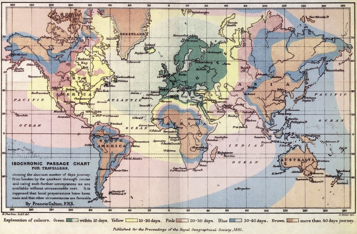
Isochrone maps may account for travel by different methods. E.g. travel by car is constrained to roads, and travel by foot is constrained (roughly) to sidewalks.
Motivation
The main idea of this project is to examine how not just density, but also the structure of roads and sidewalks impact walkability. For instance, compare these two pedestrian isochrone maps showing the destinations possible in 15 minutes of walking:
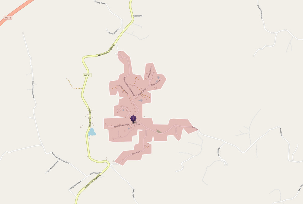
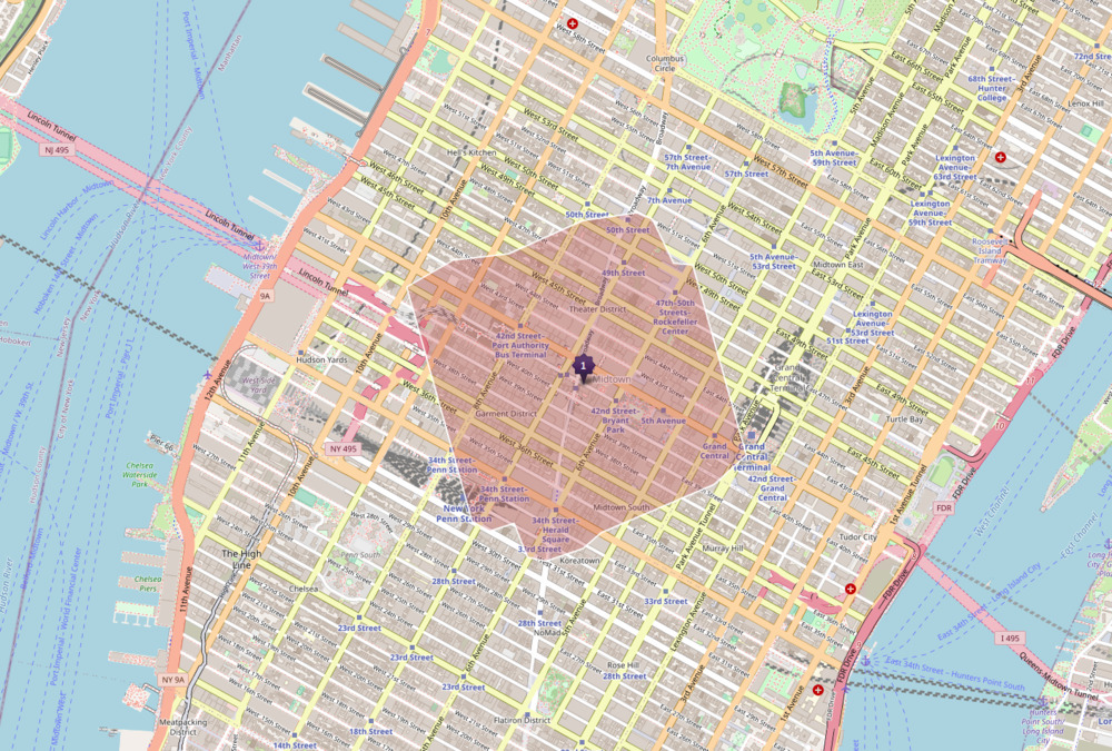
Even though there are clearly fewer amenities near this rural area, the network structure of roads also prohibits covering as much distance, not to mention the lack of sidewalks facilitating safe pedestrian travel. The city block structure in Manhattan provides a 30% increase in the walkable area from the starting point, compared to the rural area.
Valhalla
To construct isochrone maps, we'll be using a tool called Valhalla, which is an open source routing engine. This tool operates on top of openstreetmap data, which is crowdsourced by volunteers, but is generally quite thorough, especially in urban areas.
Downloading the data
First I downloaded the openstreetmap data from Geofabrik,2 which graciously hosts up-to-date extracts of openstreetmap for download.
Initially I used an extract specifically for Virginia which was a modest size of 342 MB. But after this code was tested, I ran imported the entire United States extract, which is 8.5 GB.
Then I copied the data to data/data.osm.pbf
Setting up Valhalla and PostGIS
I used docker compose to manage Valhalla and PostGIS so that I didn't have to install it locally.
For Valhalla, this docker compose file just exposes port 8002 for the API in addition to some volume mounts for the run script and the OSM data.
version: "3.9"
services:
  valhalla:
    image: valhalla/valhalla:run-latest
    ports:
      - "8002:8002"
    volumes:
      - ./scripts:/scripts
      - ./data:/data
    entrypoint: /scripts/build_tiles.sh
Combined with a simple bash script to build the Valhalla tiles and run the server:
#!/bin/bash

mkdir /data/valhalla_tiles

if ! test -f "/data/valhalla.json"; then
    echo "Valhalla JSON not found. Creating config."
    valhalla_build_config --mjolnir-tile-dir /data/valhalla_tiles --mjolnir-tile-extract /data/valhalla_tiles.tar --mjolnir-timezone /data/valhalla_tiles/timezones.sqlite --mjolnir-admin /data/valhalla_tiles/admins.sqlite > /data/valhalla.json
fi

if ! test -f "/data/valhalla_tiles/timezones.sqlite"; then
    echo "Valhalla tiles not found. Building now."
    valhalla_build_timezones > /data/valhalla_tiles/timezones.sqlite
    valhalla_build_tiles -c /data/valhalla.json /data/data.osm.pbf
fi

if ! test -f "/data/valhalla_tiles.tar"; then
    echo "Tile extract not found. Extracting now."
    valhalla_build_extract -c /data/valhalla.json -v
fi

echo "Starting valhalla server."
valhalla_service /data/valhalla.json 1
The full code can be found here.
Setting up PostGIS
PostGIS is a geospatial extension on top of PostgreSQL, which does some very cool optimizations to support efficient geospatial queries.
Similarly, I set up PostGIS using my osm2pgsql-docker repo
and imported the US dataset with osm2pgsql, a tool used for ingesting the protobuf formatted data into PostGIS.
version: "3.9"  # optional since v1.27.0
services:
  postgis:
    container_name: postgis
    image: postgis/postgis
    ports:
      - "15432:5432"
    environment:
      - POSTGRES_PASSWORD=password
    volumes:
      - type: bind
        source: ./postgresql.conf
        target: /etc/postgresql.conf
    command: ["postgres", "-c", "config_file=/etc/postgresql.conf"]
After PostGIS was running, I imported the data. This was initially tested on the Virginia state osm.pbf data,
but I later updated this to use the entire US dataset. After making this change, the script kept running out of memory.
So I added the --slim --drop flags, which process the data using PostgresSQL (using my SSD), rather than storing everything in memory.
Although I was running this on a 16 GB machine, I did not have enough free memory to process for the whole file.
PGPASSWORD=password osm2pgsql \
  --create \
  --verbose \
  -P 15432 -U postgres -H localhost \
  -S osm2pgsql.style \
  --slim --drop \
  /home/wcedmisten/Downloads/us-latest.osm.pbf
I also used a simplified version of osm2pgsql.style to reduce the number of features imported into
the database.
These 3 lines were retained, but most other tags were set to be deleted, rather than imported.
node,way   amenity      text         polygon
node,way   shop         text         polygon
node,way   leisure      text         polygon
I intentionally limited my analysis to amenity, shop, and leisure tags.
Due to using my SSD instead of memory for the import, the whole process took around 6 hours. I just let it run overnight, so this wasn't a huge issue.
Even with this reduced set of tags, the database still took up 25 GB of storage, much more than could fit in memory.
Writing the Code
Now that the backends were set up, I could begin writing the code to measure walkability. My code was intended to do several things for each city we want to measure:
- Sample some points randomly inside a city
- Find the isochrone map for each of these points within a 15 minute walk
- Find the amenities within this isochrone boundary (e.g. restaurants, parks, grocery stores, etc.)
Getting the City Boundary Data
To find the boundaries for US cities, I downloaded a few different datasets for cities:
- geoJSON files for each city's boundary for major cities in the US. These were based on the TIGER US census dataset that someone converted to GeoJSON
- top 1,000 most populous cities. I examined the top 100 cities in this dataset to compare walkability.
I then created a PostGIS table, city, to store the GeoJSON boundaries for these 100 cities using a python script:
upload_cities.py:
import psycopg2
import json

from util import get_cities

conn = psycopg2.connect(host="localhost", port="15432", dbname="postgres", user="postgres", password="password")
cur = conn.cursor()

create_city_table = """CREATE TABLE IF NOT EXISTS city (
    name text,
    state text,
	geom geometry,
    PRIMARY KEY (name, state)
);
"""

cur.execute(create_city_table)
conn.commit()


def import_city(city, state):
    with open(f"geojson-us-city-boundaries/cities/{state}/{city}.json") as f:
        data = json.load(f)

    geom = data['features'][0]['geometry']

    cur.execute("INSERT INTO city (name, state, geom) VALUES (%s, %s, %s)", (city, state, json.dumps(geom)))
    conn.commit()


# get_cities() just munged the city population JSON data to get the top 100
for city, state in get_cities():
    # print(city,state)
    import_city(city, state)
This allowed me to query whether or not a point is inside a city with the SQL query:
SELECT ST_Contains(geom, ST_GeomFromText('POINT(%s %s)'))
    FROM ( SELECT geom FROM city WHERE name=%s AND state=%s ) as geom
Sampling
I wanted to generate an even distribution of points across a city and sample "walkability" at each of these points. Then, all samples could be averaged out.
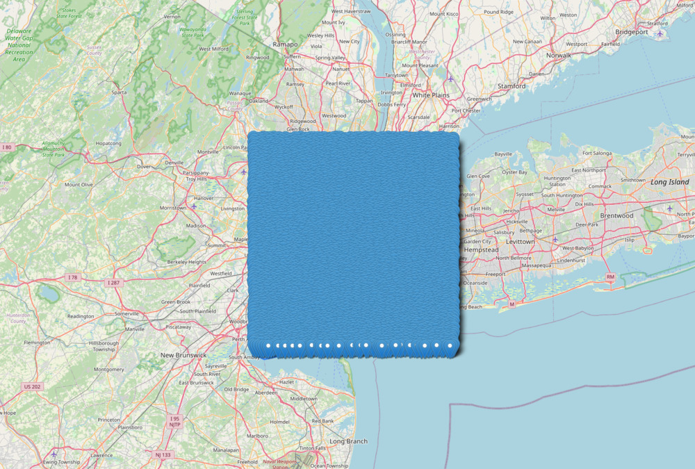
To accomplish this, I calculated the bounding box for each city, and generated a Poisson disk sampling3 of points. This distribution guaranteed minimal overlap of points being sampled.
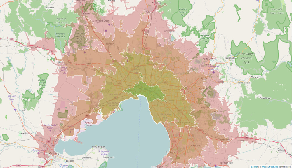
This bounding-box distribution for New York City looked like this:
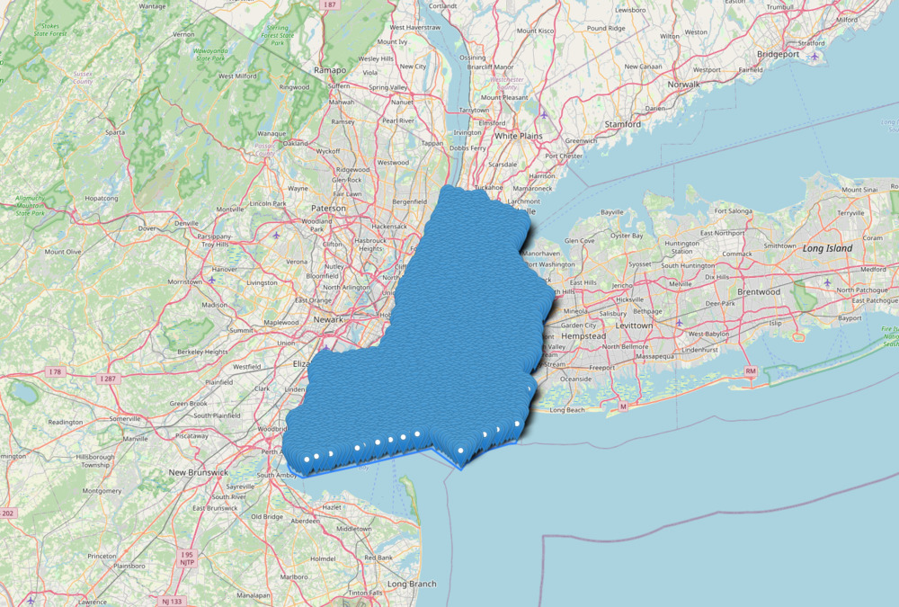
After removing the points outside of the city's actual boundaries, the sample looked like this:
Zoomed in further:
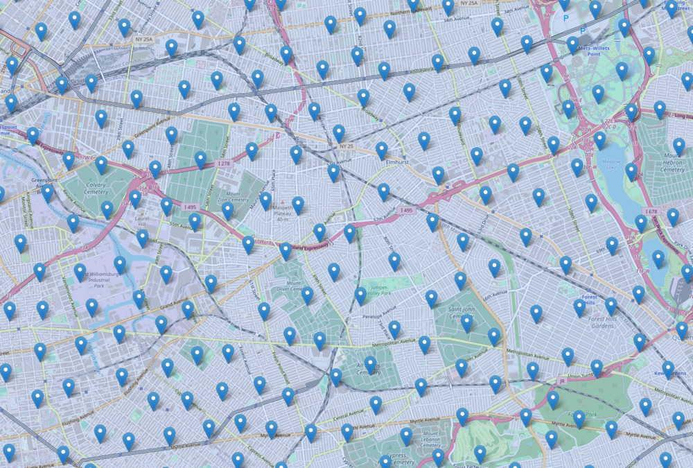
Poisson disk distributions guarantee a minimum separation distance for all the points. I picked a distance somewhat arbitrarily that would have some overlap of walkable amenities for neighboring samples, but not too much.
The code to do this was also fairly simple, relying on a library poisson_disc 4 to calculate the sample points,
and PostGIS to determine whether each point was in the city.
get_bbox_query = """SELECT ST_AsText(ST_Envelope( geom ))
FROM ( SELECT geom FROM city WHERE name=%s AND state=%s ) as geom
"""

cur.execute(get_bbox_query, [city, state])
bbox = cur.fetchone()

minx, miny, maxx, maxy = shapely.wkt.loads(bbox[0]).bounds
height = (maxy - miny)
width = (maxx - minx)

points = poisson_disc.Bridson_sampling(dims=np.array([width,height]), radius=.005)

is_in_query = """
SELECT ST_Contains(geom, ST_GeomFromText('POINT(%s %s)'))
FROM ( SELECT geom FROM city WHERE name=%s AND state=%s ) as geom
"""

scaled = list(map(lambda p: [p[0] + minx, p[1] + miny], points))

def point_in_city(point):
    is_in_city = cur.execute(is_in_query, [point[0], point[1], city, state])
    return cur.fetchone()[0]

# get all the points in the given city
in_city = list(filter(point_in_city, scaled))
Creating a metric
Now that I had a sampling for the city, I needed a metric to calculate for each point.
I used a relatively simple approach: I examined a few categories of urban amenities and gave 1 point to each unique category of amenity within a 15 minute walking distance. The walking distance was determined by querying Valhalla for each sampled point.
For instance, a point with 3 restaurants, 2 bakeries, and 1 shoe store within walking distance would get a score of 3: 1 point for each category. I reasoned that most amenities are essentially a binary category. Either the amenity you want is within walking distance or it's not. For future work, I would probably change this to a logarithmic or logistic function to reflect diminishing returns on amenities of the same category.
The first bakery within walking distance provides much more value than the second one, which provides more value than the third, etc.
It was also simpler to examine these categories at a binary level because the OSM data model has many places where a single entity would be represented as multiple nodes (i.e. a building polygon), and this approach avoided that complexity.
15 minutes was chosen somewhat arbitrarily, but is about the maximum I would consider to be a "quick walk" to a destination. In the future, this could be explored using variable distances per amenity.
I created a function get_amenities(lat, lon) to retrieve the amenities within walking distance of a point.
MAX_WALK_TIME = 15

def get_amenities(lat, lon):
    payload = {
        "locations":[
            {"lat": lat,"lon": lon}
        ],
        "costing":"pedestrian",
        "denoise":"0.11",
        "generalize":"0",
        "contours":[{"time":MAX_WALK_TIME}],
        "polygons":True
    }


    request = f"http://localhost:8002/isochrone?json={json.dumps(payload)}"
    isochrone = requests.get(request).json()

    geom = json.dumps(isochrone['features'][0]['geometry'])

    query = f"""
    SELECT * FROM planet_osm_point
    WHERE ST_Contains(ST_Transform(ST_GeomFromGeoJSON('{geom}'),3857), way) AND (amenity IS NOT NULL OR shop IS NOT NULL OR leisure IS NOT NULL);
    """

    cur.execute(query)
    rows = cur.fetchall()

    cur.execute("SELECT * FROM planet_osm_point LIMIT 0")
    colnames = [desc[0] for desc in cur.description]

    return to_dict(colnames, rows)
This function:
- makes a request to the Valhalla Isochrone service to get the polygon representing a 15 minute walk surrounding the point
- uses that polygon to find all unique amenities within those bounds
The amenities considered here are represented in the following OSM tags, including their definitions from the OSM wiki.
amenity:cafe- a generally informal place with sit-down facilities selling beverages and light meals and/or snacksamenity:bar- a purpose-built commercial establishment that sells alcoholic drinks to be consumed on the premisesamenity:pub- an establishment that sells alcoholic drinks that can be consumed on the premisesamenity:restaurant- formal eating places with sit-down facilities selling full meals served by waitersshop:bakery- a shop selling breadshop:convenience- a small local shop carrying a variety of everyday products, mostly including single-serving food itemsshop:supermarket- a large shop for groceries and other goods, including meat and fresh produceshop:department_store- a large store with multiple clothing and other general merchandise departmentsshop:clothes- a shop which primarily sells clothing, such as underwear, shirts, jeans etcshop:shoes- is a type of retailer that specialises in selling shoesshop:books- A shop selling books (including antique books, chain bookstores, etc.)shop:hairdresser- where you can get your hair cutleisure:fitness_center- a place with exercise machines and/or fitness/dance classes. They are places to go to for exerciseleisure:park- an area of open space for recreational use, usually designed and in semi-natural state with grassy areas, trees and bushes
Results
Top 10 most walkable cities
| Rank | City | Amenity Score |
|---|---|---|
| 1 | washington-dc dc | 5.54 |
| 2 | minneapolis mn | 4.31 |
| 3 | chicago il | 4.2 |
| 4 | new-york ny | 4.07 |
| 5 | seattle wa | 4.01 |
| 6 | cleveland oh | 3.84 |
| 7 | denver co | 3.37 |
| 8 | jersey-city nj | 3.31 |
| 9 | st-louis mo | 3.14 |
| 10 | pittsburgh pa | 3.07 |
Least 10 walkable cities:
| Rank | City | Amenity Score |
|---|---|---|
| 91 | louisville-jefferson ky | 0.39 |
| 92 | tucson az | 0.38 |
| 93 | north-las-vegas nv | 0.36 |
| 94 | jacksonville fl | 0.35 |
| 95 | lubbock tx | 0.32 |
| 96 | oklahoma-city ok | 0.31 |
| 97 | chesapeake va | 0.27 |
| 98 | bakersfield ca | 0.22 |
| 99 | corpus-christi tx | 0.17 |
| 100 | anchorage ak | 0.05 |
I also compared these rankings to Walk Score, and found that they seemed to be mostly in the ballpark.
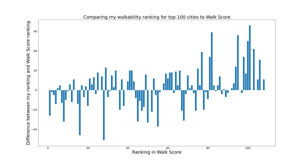
This plot shows the difference between the Walk Score ranking and my ranking. E.g. I ranked San Fransisco as #26, but Walk Score ranked it at #1, showing a bar at -25 for the first entry. The x axis is ordered by the walk score ranking.5
Limitations
Some significant limitations:
- I didn't filter samples that aren't on land
- I didn't filter for residential areas (although arguably this could be intentional to count tourism and travel)
- openstreetmap is made by crowdsourced data from volunteers, and amenity data may not be evenly distributed (probably benefitting higher population cities)
- Biases from the boundaries of the city vs. metropolitan sprawl. This would be biased toward larger metropolitan areas
Performance
I profiled running this on a single city with flameprof6, and found that the majority of time is spent between querying Valhalla and querying PostGIS, which makes sense to me. Both Valhalla and PostGIS are most likely heavily optimized already, so the only way I could shave down runtime would be to sample fewer points.

Future Work
Custom walkability scores
Explore customized walkability scores. "Walkability" based on all amenities is painting with a broad brush. Most people probably don't care about every single amenity that can be categorized. Peter Johnson has an interesting article7 about reverse engineering the Walk Score, which found that it's highly correlated with the number of nearby restaurants.
Personally, I love restaurants, but I cook most of my meals at home, so this score may be less useful to me. I like the idea of assigning weights to each amenity to get a more custom optimization. You could even optimize for something like "most walkable Chinese restaurants" or "most parts".
We could also codify some other factors with walkability related to the isochrone calculations. For example, people with disabilities may have an especially hard time with poor sidewalk infrastructure. I don't think Valhalla supports custom sidewalk cost penalties related to width, sidewalk condition, or curb cuts, but I would be interested in exploring that more specifically.
One of the coolest things about openstreetmap is the level of detail available in the data. I don't know of anywhere else where curb cut data is available.
Amenity centered isochrones
Another idea I had was instead of sampling a bunch of points, which requires a lot of isochrone calculations, instead calculate isochrones starting from each amenity. Then we could combine all the isochrone polygons and calculate what portion of the city is within X minute walk of that amenity. This could also be useful for finding amenity "deserts", like food deserts, but more general.
This would also allow me to explore varying the walking distance for each amenity category. E.g. I would be more willing to walk further for infrequent and important errands, like electronics repair or a hospital visit. But for more common tasks like getting groceries, I would prefer a closer walk.
Appendix
Source Code:
https://github.com/wcedmisten/city-walkability
https://github.com/wcedmisten/osm2pgsql-docker
Final Rankings
| Rank | City | Amenity Score |
|---|---|---|
| 1 | washington-dc dc | 5.54 |
| 2 | minneapolis mn | 4.31 |
| 3 | chicago il | 4.2 |
| 4 | new-york ny | 4.07 |
| 5 | seattle wa | 4.01 |
| 6 | cleveland oh | 3.84 |
| 7 | denver co | 3.37 |
| 8 | jersey-city nj | 3.31 |
| 9 | st-louis mo | 3.14 |
| 10 | pittsburgh pa | 3.07 |
| 11 | philadelphia pa | 3.0 |
| 12 | portland or | 2.94 |
| 13 | st-paul mn | 2.87 |
| 14 | san-jose ca | 2.8 |
| 15 | buffalo ny | 2.67 |
| 16 | baltimore md | 2.63 |
| 17 | detroit mi | 2.57 |
| 18 | boston ma | 2.55 |
| 19 | oakland ca | 2.54 |
| 20 | miami fl | 2.44 |
| 21 | sacramento ca | 2.4 |
| 22 | omaha ne | 2.33 |
| 23 | chandler az | 2.26 |
| 24 | long-beach ca | 2.11 |
| 25 | santa-ana ca | 2.04 |
| 26 | madison wi | 2.01 |
| 27 | san-francisco ca | 2.0 |
| 28 | milwaukee wi | 1.91 |
| 29 | los-angeles ca | 1.9 |
| 30 | richmond va | 1.89 |
| 31 | cincinnati oh | 1.89 |
| 32 | san-diego ca | 1.83 |
| 33 | chula-vista ca | 1.8 |
| 34 | atlanta ga | 1.8 |
| 35 | gilbert az | 1.76 |
| 36 | honolulu hi | 1.76 |
| 37 | anaheim ca | 1.76 |
| 38 | mesa az | 1.74 |
| 39 | raleigh nc | 1.64 |
| 40 | newark nj | 1.64 |
| 41 | lincoln ne | 1.62 |
| 42 | albuquerque nm | 1.51 |
| 43 | las-vegas nv | 1.49 |
| 44 | austin tx | 1.43 |
| 45 | columbus oh | 1.4 |
| 46 | plano tx | 1.34 |
| 47 | colorado-springs co | 1.34 |
| 48 | aurora co | 1.33 |
| 49 | st.-petersburg fl | 1.3 |
| 50 | greensboro nc | 1.29 |
| 51 | riverside ca | 1.28 |
| 52 | houston tx | 1.25 |
| 53 | boise-city id | 1.24 |
| 54 | tampa fl | 1.24 |
| 55 | glendale az | 1.19 |
| 56 | fremont ca | 1.1 |
| 57 | toledo oh | 1.07 |
| 58 | irvine ca | 1.04 |
| 59 | stockton ca | 1.03 |
| 60 | orlando fl | 1.01 |
| 61 | charlotte nc | 1.0 |
| 62 | hialeah fl | 0.99 |
| 63 | indianapolis-city in | 0.99 |
| 64 | durham nc | 0.96 |
| 65 | norfolk va | 0.96 |
| 66 | phoenix az | 0.9 |
| 67 | baton-rouge la | 0.88 |
| 68 | dallas tx | 0.84 |
| 69 | reno nv | 0.83 |
| 70 | fort-wayne in | 0.82 |
| 71 | arlington tx | 0.8 |
| 72 | wichita ks | 0.77 |
| 73 | garland tx | 0.75 |
| 74 | irving tx | 0.75 |
| 75 | winston-salem nc | 0.71 |
| 76 | tulsa ok | 0.69 |
| 77 | fresno ca | 0.67 |
| 78 | kansas-city mo | 0.67 |
| 79 | new-orleans la | 0.66 |
| 80 | fort-worth tx | 0.65 |
| 81 | san-antonio tx | 0.58 |
| 82 | henderson nv | 0.58 |
| 83 | san-bernardino ca | 0.56 |
| 84 | nashville-davidson-metropolitan-government tn | 0.55 |
| 85 | memphis tn | 0.54 |
| 86 | scottsdale az | 0.53 |
| 87 | lexington-fayette ky | 0.51 |
| 88 | el-paso tx | 0.48 |
| 89 | laredo tx | 0.44 |
| 90 | virginia-beach va | 0.4 |
| 91 | louisville-jefferson ky | 0.39 |
| 92 | tucson az | 0.38 |
| 93 | north-las-vegas nv | 0.36 |
| 94 | jacksonville fl | 0.35 |
| 95 | lubbock tx | 0.32 |
| 96 | oklahoma-city ok | 0.31 |
| 97 | chesapeake va | 0.27 |
| 98 | bakersfield ca | 0.22 |
| 99 | corpus-christi tx | 0.17 |
| 100 | anchorage ak | 0.05 |